Multi-Agent AI Systems Tackle Personal Finance
IMPORTANT DISCLAIMER
This article describes an experimental AI system for demonstration only. I am not a financial advisor. All examples use simplified models with hypothetical data. Consult qualified professionals before making financial decisions.
Introduction
 Image generated by author using GPT-4o
Personal finance decision making often involves various multi-faceted problems: evaluating investments like stocks and ETFs, determining retirement allocations, or evaluating savings rates. However, comprehensively considering all vital factors is challenging. This motivated me to explore AI not just for isolated answers but for automating the end-to-end financial research and analysis process. This post describes an experiment using specialized AI agents, orchestrated to work together and provide more comprehensive insights than a single Large Language Model (LLM) might provide alone.
The Promise of AI Agent Orchestration
Recent AI advancements favor systems of specialized agents collaborating on complex tasks over monolithic models. Frameworks like Autogen, CrewAI, and LangGraph facilitate this multi-agent approach, enabling more sophisticated problem-solving via orchestration: the management of agent communication, context, and task execution allowing agents to build upon each other’s work in cohesive workflows.
My Experiment: A Financial Planning Agent System
To investigate the potential of agent orchestration for financial tasks, I developed a proof-of-concept system using Autogen’s MagenticOne [1] framework, specifically the MagenticOneGroupChat. MagenticOne was selected for its sophisticated orchestration mechanism, designed to maintain high-level strategic awareness and detailed tactical control throughout complex workflows.
System Architecture
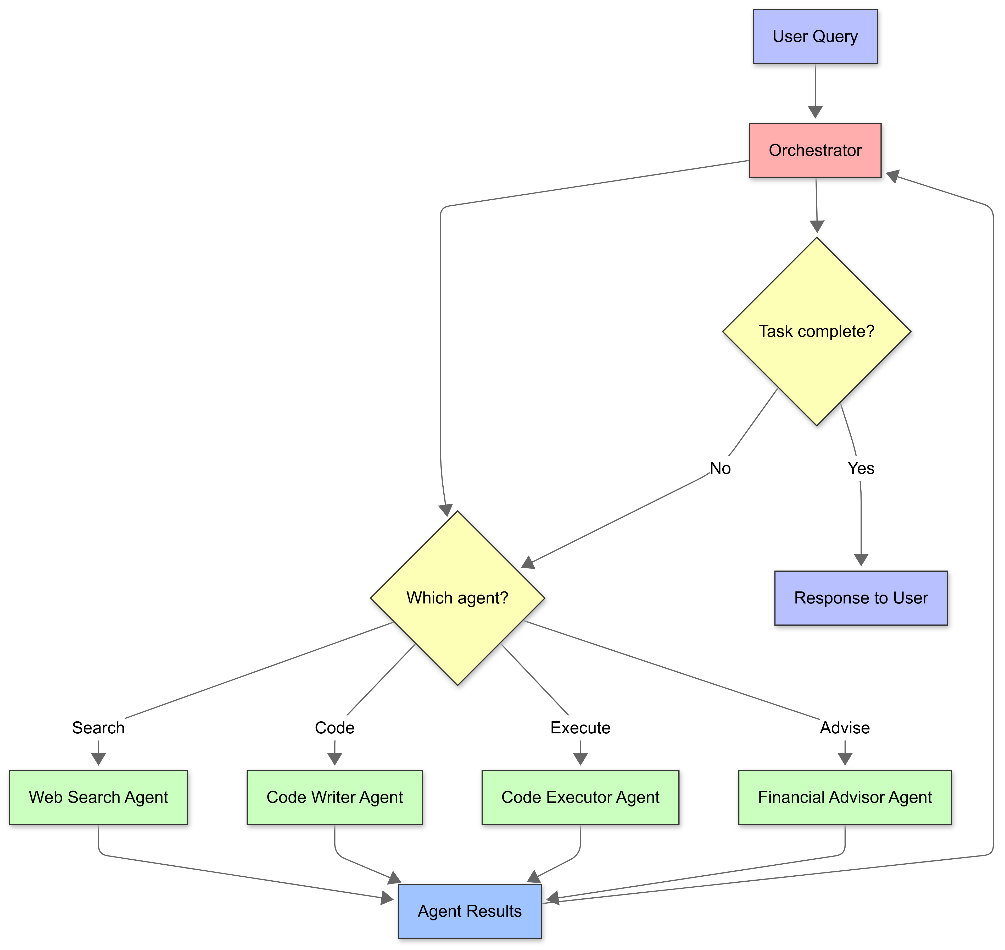 AI Agent Orchestration: How specialized agents collaborate under central coordination to solve complex user queries (image by author)
The system utilizes four specialized agents, each handling a specific financial planning aspect:
-
🔍 Web Search Agent: Retrieves current financial data by querying the Perplexity search API. It summarizes the returned search results and formats the key findings for downstream use.
-
💻 Code Writer Agent: Generates Python algorithms for financial calculations (e.g., retirement projections, portfolio analysis). It focuses on producing well-documented, error-handled code.
-
⚙️ Code Executor Agent: Executes the generated Python code snippets and returns computational results.
-
📊 Financial Advisor Agent: Synthesizes retrieved information and computational results into actionable recommendations, applying financial planning principles.
Orchestration Mechanics (MagenticOne)
The MagenticOne orchestrator coordinates these agents via a structured process:
-
Fact Sheet Creation: Deconstructs the user’s query into a fact sheet (Given/verified facts, Facts to look up, Facts to derive, Educated guesses).
-
Sequential Planning: Develops a step-by-step plan, assigning tasks to the appropriate agent.
-
Dual-Ledger Management: During execution, it maintains two ledgers:
- Task Ledger for strategic planning and tracking progress.
- Progress Ledger for detailed, step-by-step task execution and completion logs.
This dual-ledger method ensures high-level logical planning and tactical effectiveness, directing each agent when needed.
The System in Action
Let’s examine how this system handles real financial planning questions through two examples:
Example 1: Retirement Planning Analysis
Scenario: A 40-year-old user wants to retire at 65. They have $150,000 in a 401(k), earn $95,000 annually, contribute 8% (plus a 3% employer match), and have a moderate risk tolerance. They asked for advice on contribution rates and allocation, retirement projections, and a safe withdrawal rate (SWR) analysis.
1. Orchestrator: Fact Sheet & Plan
The orchestrator structured the query (Given facts, Facts to look up, Facts to derive, Educated guesses) and planned the task sequence, starting with data retrieval.
2. Web Search Agent: Data Retrieval
This agent used the Perplexity API to find key data points (example data fetched by perplexity as of February 2025):
Market & Economic Data:
- Moderate-risk (60/40) portfolio returns: Avg. 6.9% annually (past decade); range 6-8.8%.
- Inflation: 2.8%; projected 2.4-2.6%.
- 401(k) fees: Avg. 0.5-1% (large plans), 1-2% (small plans).
- Safe Withdrawal Rate (SWR): Updated consensus around 3.7% (down from 4%).
The agent summarized and formatted these findings.
3. Code Writer Agent: Projection Model
The Code Writer Agent generated Python code for projections, incorporating user profile and web search data:
# AI agent generated
# Import necessary libraries
import numpy as np

# Constants and initial values
current_age = 40
retirement_age = 65
years_to_retirement = retirement_age - current_age

# Financial details
current_balance = 150000      # Current 401(k) balance
annual_income = 95000         # Current annual income
contribution_rate = 0.08      # 8% personal contribution
employer_match_rate = 0.03    # 3% employer match
annual_return_rate = 0.069    # 6.9% annual return
inflation_rate = 0.028        # 2.8% inflation rate (as of February 2025)
annual_fees = 0.0075          # 0.75% annual fees
salary_growth_rate = 0.025    # 2.5% annual salary growth
safe_withdrawal_rate = 0.037  # 3.7% safe withdrawal rate

# Calculate annual contributions
def calculate_annual_contribution(income, contribution_rate, employer_match_rate):
    personal_contribution = income * contribution_rate
    employer_contribution = income * employer_match_rate
    return personal_contribution + employer_contribution

# Project 401(k) balance at retirement
def project_401k_balance(current_balance, annual_contribution, years,
                        annual_return_rate, annual_fees, salary_growth_rate):
    balance = current_balance
    for year in range(years):
        # Apply salary growth
        annual_contribution *= (1 + salary_growth_rate)
        # Calculate annual growth
        balance = balance * (1 + annual_return_rate - annual_fees) + annual_contribution
    return balance

# Calculate monthly withdrawal amount
def calculate_monthly_withdrawal(balance, safe_withdrawal_rate):
    annual_withdrawal = balance * safe_withdrawal_rate
    return annual_withdrawal / 12

# Calculate initial annual contribution
initial_annual_contribution = calculate_annual_contribution(
    annual_income, contribution_rate, employer_match_rate
)

# Project the 401(k) balance at retirement
projected_balance = project_401k_balance(
    current_balance, initial_annual_contribution, years_to_retirement,
    annual_return_rate, annual_fees, salary_growth_rate
)

# Calculate the monthly withdrawal amount
monthly_withdrawal = calculate_monthly_withdrawal(
    projected_balance, safe_withdrawal_rate
)

# Print results
print(f"Projected 401(k) balance at age {retirement_age}: ${projected_balance:,.2f}")
print(f"Monthly withdrawal amount at retirement (using {safe_withdrawal_rate*100:.1f}% safe withdrawal rate): ${monthly_withdrawal:,.2f}")
4. Code Executor Agent: Calculation
The Code Executor Agent ran the code and returned the results:
Projected 401(k) balance at age 65: $1,427,700.37
Monthly withdrawal amount at retirement (using 3.7% safe withdrawal rate): $4,402.08
5. Financial Advisor Agent: Synthesis & Recommendations
The Financial Advisor Agent looked at all the messages till now and provided tailored recommendations:
AI agent generated
Contribution Rate Recommendation: Your current 11% total contribution is solid, projecting ~$1.43 million. Increasing personal contributions towards 10-12% would significantly enhance retirement security if feasible within your budget.
Investment Allocation Recommendation: Maintain a diversified portfolio aligned with moderate risk. Given the 25-year horizon, an allocation of roughly 60-70% stocks and 30-40% bonds is appropriate. Ensure low-cost index funds are used.
Withdrawal Strategy: The projected ~$4,402 monthly withdrawal (based on a 3.7% SWR from ~$1.43M) provides a reasonable baseline. This needs to be considered alongside expected Social Security benefits and potential part-time income or other assets. The 3.7% SWR is a conservative starting point derived from recent studies.
Additional Recommendations:
- Rebalance the portfolio annually to maintain the target allocation.
- Ensure you have a separate emergency fund (3-6 months of expenses) outside your 401(k).
- Remember that the projection uses an average return; actual returns will vary. Inflation (estimated at 2.8% currently) will erode purchasing power.
- Consider strategies for maximizing Social Security benefits, potentially by delaying claims if possible.
Outcome: This example highlights the orchestrator directing specialized agents to perform specific tasks. The Web Search Agent’s findings informed the Code Writer’s parameters. The code results, along with the web search results, formed the basis for the Financial Advisor’s analysis. This resulted in an integration of up-to-date data with projections, a task challenging for a single model.
Example 2: Portfolio Optimization
Scenario: A user asked for advice on allocating $50,000 across VOO, VXUS, BND (Vanguard ETFs), with moderate risk tolerance and a 5+ year horizon.
1. Orchestrator: Fact Sheet & Plan
The orchestrator structured the query (knowns, lookups, derivations, guesses) and planned a four-step process for the agents.
2. Web Search Agent: Data Retrieval
The agent retrieved ETF data (example data fetched by perplexity as of March 2025):
| ETF | Expense Ratio | 3-Year Avg Annual Return |
|---|---|---|
| VOO | 0.03% | 9.0% |
| VXUS | 0.05% | 2.19% |
| BND | 0.03% | 0.09% |
Vanguard’s Recommended Moderate Allocation: ~50-55% Stocks, ~45-50% Bonds
3. Code Writer Agent: Portfolio Analysis
The agent generated a Modern Portfolio Theory optimization model:
# AI agent generated
import numpy as np
import pandas as pd
import matplotlib.pyplot as plt

# Define expected returns and volatilities
returns = np.array([0.09, 0.0219, 0.0009])      # VOO, VXUS, BND
volatilities = np.array([0.15, 0.17, 0.05])      # VOO, VXUS, BND

# Define correlation matrix (typical estimates for these asset classes)
# VOO/VXUS (US/Intl Stock) - High correlation
# VOO/BND (US Stock/Bond) - Low/Negative correlation
# VXUS/BND (Intl Stock/Bond) - Low/Negative correlation
correlation_matrix = np.array([
    [1.0,  0.85, -0.2],
    [0.85, 1.0,  -0.1],
    [-0.2, -0.1,  1.0]
])

# Calculate covariance matrix
covariance_matrix = np.outer(volatilities, volatilities) * correlation_matrix

# Function to calculate portfolio performance
def portfolio_performance(weights, returns, covariance_matrix):
    portfolio_return = np.dot(weights, returns)
    portfolio_volatility = np.sqrt(
        np.dot(weights.T, np.dot(covariance_matrix, weights))
    )
    return portfolio_return, portfolio_volatility

# Function to generate random portfolios
def generate_portfolios(num_portfolios, returns, covariance_matrix):
    results = np.zeros((3, num_portfolios))
    weights_record = []

    for i in range(num_portfolios):
        weights = np.random.random(len(returns))
        weights /= np.sum(weights)
        weights_record.append(weights)

        portfolio_return, portfolio_volatility = portfolio_performance(
            weights, returns, covariance_matrix
        )
        results[0,i] = portfolio_return
        results[1,i] = portfolio_volatility
        # Sharpe Ratio (assuming risk-free rate is 0)
        results[2,i] = results[0,i] / results[1,i]

    return results, weights_record

# Generate a large number of random portfolios
num_portfolios = 10000
results, weights_record = generate_portfolios(
    num_portfolios, returns, covariance_matrix
)

# Find the optimal portfolio for moderate risk tolerance (target volatility ~10%)
target_volatility = 0.10

# Find the index of the portfolio closest to the target volatility
closest_volatility_index = np.abs(results[1,:] - target_volatility).argmin()

# Optimal weights are extracted based on 'closest_volatility_index' for execution
# Note: This represents the core portfolio optimization algorithm.
# Additional code for data preparation, and implementation details
# have been omitted for clarity and focus in this blog post.
4. Code Executor Agent: Analysis Results
The Executor Agent ran the optimization model, identifying an optimal portfolio for moderate risk (targeting ~10% volatility):
Optimal Portfolio Weights for Moderate Risk Tolerance (Target Volatility ~10%):
VOO: 65.16%
VXUS: 2.86%
BND: 31.98%

Expected Portfolio Return: 5.96%
Expected Portfolio Volatility: 10.00%
5. Financial Advisor Agent: Recommendations
The Advisor Agent synthesized results into actionable and specific guidance:
AI agent generated
Recommended Allocation ($50,000): Based on the analysis targeting approximately 10% annual volatility suitable for moderate risk tolerance over 5+ years:
- VOO (Vanguard S&P 500 ETF): $32,580 (65.16%) - Provides core U.S. equity exposure.
- VXUS (Vanguard Total Intl Stock ETF): $1,430 (2.86%) - Adds international diversification.
- BND (Vanguard Total Bond Market ETF): $15,990 (31.98%) - Reduces overall portfolio volatility and provides stability.
Guidance:
- Establish Initial Allocation: Invest the $50,000 according to these percentages.
- Rebalance Periodically: Check the portfolio annually or semi-annually. If the allocations drift significantly (e.g., by more than 5%) due to market movements, sell some of the overweight asset(s) and buy the underweight one(s) to return to the target weights.
- Stay Disciplined: Long-term investing requires patience. Avoid making drastic changes based on short-term market noise. This allocation is designed for a 5+ year horizon.
Outcome: This demonstrates the system incorporating market data, quantitative analysis (MPT), and investment principles to illustrate how such a system might function. The orchestrator guided the process, with each agent performing its specialized function in a cohesive workflow.
Technical Insights
Developing this agentic system gave me several insights:
-
Planning is Important: The logical problem-solving abilities of the MagenticOne framework were impressive. Its dual-ledger method broke down problems into multiple steps while maintaining the flexibility necessary for the successful completion of each task. The orchestrator’s planning and management ensured a smooth flow of information.
-
Specialization is Good: The system allowed us to optimize each agent for its role. This enabled us to reduce prompt complexity and improve reliability.
-
Community Learning: Each agent’s insights informed other agents, as they had access to the relevant context in each run. This information sharing was critical to developing a cohesive solution to the user query.
-
Multi-Model Approach: The system allows using different LLMs across agents rather than relying on a single model. I chose Claude 3.5 Sonnet as the orchestrator for its strong reasoning capabilities, while deploying GPT-4o for specialized agents (Web Search, Code Writer, Financial Advisor). This shows the system’s flexibility - users can choose the model to suit specific requirements or even incorporate fine-tuned LLMs to achieve better accuracy for domain-specific tasks.
Challenges and Limitations
Building this system revealed significant challenges:
-
Accuracy Risk: A personal and important field like financial advice demands a high level of accuracy. Reducing or eliminating hallucinations and guaranteeing factual correctness remains a significant challenge in the field of LLMs. The system relies on the perplexity search API quality and LLM interpretation, requiring careful user scrutiny.
-
Simple Financial Modeling: Currently, based on empirical observations, the system leans on idealized models and simple calculations. While reasonable for many scenarios, this might not capture the complexity of financial markets. Financial analysis is inherently an uncertain domain, contingent on many factors. Often, the system presented here uses point estimates rather than probabilistic techniques, giving users a false sense of precision. More sophisticated approaches incorporating scenario analysis and risk modeling would better represent the range of possible outcomes in financial planning.
Conclusion
This experiment illustrates that AI agents working in collaboration can successfully tackle complex tasks like financial planning. When we have different AI tools working together - one searching the web, another writing code, a third running calculations, and a fourth analyzing financial information - we can provide deeper insights than a single LLM can provide.
While this is a promising start, it’s essential to acknowledge the system’s limitations. As of now, the system does not have the ability to handle follow-up messages, so enabling this should allow users to better understand all possible options as well as clarify recommendations.
Future enhancements can also include:
- A “Fact Checker” agent as an accuracy guardrail
- Robust validation of generated code before execution (check if libraries exist in the environment?)
- Access to more exclusive sources of financial data
- A Visualization agent to create intuitive charts of projections
- Probabilistic simulation capabilities to better represent market uncertainty
With these improvements, this agent orchestration approach could make financial planning more accessible while maintaining the nuance and personalization that financial decisions require.
Lastly, in my opinion, even as these agentic systems get more advanced and reliable for tackling complex tasks, the role of human oversight - especially when it comes to this experiment (money decisions) - remains crucial.
References
[1] A. Fourney et al., Magentic-One: A Generalist Multi-Agent System for Solving Complex Tasks (2024), arXiv:2411.04468 [cs.AI]. https://arxiv.org/abs/2411.04468
Final Reminder: The system described is an experimental demonstration, not a financial advisory tool. The examples are hypothetical and rely on simplified models. Readers should consult with a qualified professional before making financial decisions.